Utilizing the data gathered from your external Cisco Meeting Server (‘CMS’) and VCS Expressway E and C devices
Introduction
Before reading this Documentation, make sure you have gone through the setup chapter to enable the data to be ingested in Elasticsearch.
In this chapter, we will explain how to utilize the data gathered from your external Cisco Meeting Server (‘CMS’) and VCS Expressway E and C devices (collectively described as ‘Expressway’ in this document).
This functionality is currently in beta, and will undergo changes in the future, aiming at a complete feature release in a future version.
Some of the visualisations you can now find in Kibana are subject to changes, and you might want to edit/add visualisations yourself.
Any feedback and suggestions will be appreciated and will allow us to improve the user experience, please send it at tescobar@vqcomms.com.
We will now explain what data from your external monitoring you can currently find in Kibana, and how to utilize it best.
How is data structured in Elasticsearch
Before thinking of utilizing the data, it is important to have a basic understanding on how it’s structured and stored.
The smaller unit of data in Elasticsearch is a Field.
In a conventional database, a field would be a single unit of data. Each field has a defined type (string, number, date, boolean), name (key) and value.
For example, there could be a field called “Username”, which would be of type String, and would contain the value “John Smith”.
The next unit of storage, which is considered the base unit, is a Document.
In a conventional database, a document would be a row in a table. A document is a JSON object that contains a number of fields, defined by their type, key and value.
Some of those fields are reserved and contain metadata, for example the _id field that represent the unique identifier for the document.
An example of a document could be:
{
   "_id": 3,
   "_source":{
   "age": 28,
   "name": ["daniel”],
   "year":1989,
}
The largest unit of data in Elasticsearch is an Index.
In a conventional database, an index would be a table. An index is a logical partition of documents. You could for example have one index containing all the data related to your products, and another with all the data related to customers.
Finally, Kibana requires an Index Pattern to access the Elasticsearch data that you want to explore.
An index pattern selects the data to use, and can point to a specific index or multiple ones. For example, if you have the following indices:
- index_customer1
- index_customer2
- index_customer3
- index_product1
- index_product2
- index_product3
…
The index pattern “index_customer*” will point to the indices that match the pattern, so the first three in this case.
External monitoring data
The data ingested from VCS and CMS are separated in four separate index patterns:
- expressway_metrics*
- expressway_cdrs*
- expressway_logs*
- cms_logs*
From those index patterns, we have created a number of Kibana visualisations, which are regrouped in four Dashboards:
- Expressway Metrics – Metrics coming in from Expressway (metric collection, collectd)
- Expressway Participants – Data coming in from Expressway CDRs regarding the calls and participants
- Expressway Logs – List of logs coming in from Expressway (syslogs)
- CMS Logs – List of logs coming in from CMS
We will now go through the different index patterns, and give a quick introduction of the data. If you want to have a look at the data yourself, the discover panel in Kibana is probably the best way to get to know your data. There, you can select the index pattern you want to dig into, select the field keys you are interested in, and then see the values for each document.
We will now use the saved searches in the discover panel to give an overview of the data present in each index pattern.
Expressway_metrics*
(Saved searches: ExpresswayMetricsDiskUsage and ExpresswayMetricsCpuUsage)
This index pattern regroups the system performance and statistics data collected from the Expressway nodes, which is gathered periodically by the daemon called Collectd.
In the screenshot below, (Fig.1), you can see the saved search ExpresswayMetricsDiskUsage opened in the Discover page.
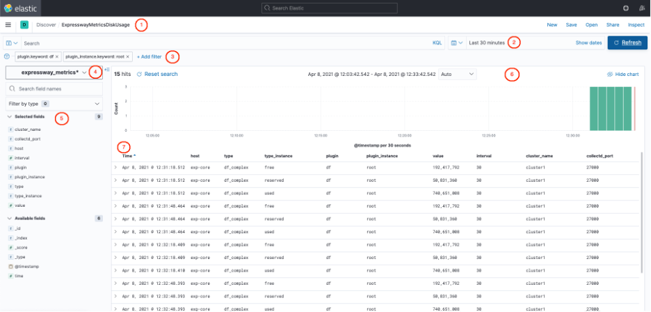
Figure 1: ExpresswayMetricsDiskUsage search in Discover
Let’s break down what is going on, from top to bottom:
- Here you can see that we are on the Discover page, and that we are looking at the ExpresswayMetricsDiskUsage search. On the right of that are the buttons to perform different actions on a search, such as create, save, and open.
- This is where the time window displayed is selected. In this case, we used the “quick select” function to select data from the last 30 minutes.
- Here is the current list of filters. You can add, remove, enable, disable and edit filters in this section. In this case, we have a filter on the keyword “plugin” to select the “df” plugin, which returns information on the amount of available disk space of the file system.
- This drop down menu allows you to select the index pattern to use for this search. Kibana will then auto-fill the available fields (5) from the documents found in the indices referenced by the index pattern.
-
This section displays all the available fields, and lets you select the ones you want to display in the table (7). On the left of each field name (known as key), you can see a symbol that represents the type of the field (e.g.; string, number, date…). If you click on a field, you can get a preview of the distribution of values for that field. In the screenshot below, (Fig. 2), you can see the distribution for the field “type_instance”, which is of type “string” for a sample of 500 documents. This shows us that a third of the documents each are related to reserved, free and used disk space.
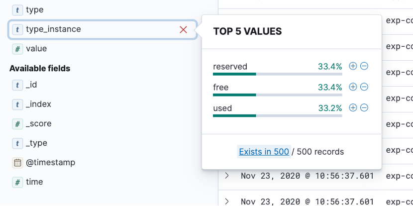
Figure 2: Distribution preview for field values
- This bar chart simply displays the number of documents (or records) found in the index pattern for the selected time window, over time. It is important to note that it takes the applied filters (3) into account.
- Finally, this table displays the list of documents found for that search, including the applied filters (3) and selected time window (2). Each line represents a document, and each column represents one of the selected fields. Here are some of the information contained in the first document of the list:
- “Time”, time the record was created: Nov 23, 2020 @ 11:00:37.601
- “host”, name of the Expressway node the data was collected from: exp-core
- “type_instance”, indicates if this record concerns free, used or reserved disk space: free
- “value”, the value measured by the plugin: 344,173,568
“cluster_name”, the name configured during the setup for that Expressway cluster: cluster1
“collectd_port”, the port configured during the setup for that Expressway cluster: 27000
NOTE: You can click on the ‘+’ next to a value in the table to create a filter on that value.
For example, clicking on the value “free” in the column “type_instance” will create a filter that will only display information about free disk space. There is also a ‘-‘ option, that will create a filter to exclude that value.
This index pattern contains collected data from many more plugins that gives us more information on the system. We currently use the plugins related to cpu, memory, disk and interface usage, but could use more in the future.
Expressway_cdrs*
(Saved searches: ExpresswayCdrsSearch, ExpresswayCdrsLegsSearch and ExpresswayCdrsChannelsSearch)
This index pattern regroups all the Call Data Records (CDRs) collected from the Expressway API from each node, through a cronjob that runs periodically. One CDR is created per participant joining a call. Considering the complexity of those records, and the amount of information contained in them, this is the most complex index pattern described in this document.
Additionally, some of the inner objects (legs and channels) contained in the main CDR object have been split into multiple documents to make it possible to access them independently. Each document contains a field called “doc_type” to identify if it contains information about a cdr, leg or channel.
Please see Example of a CDR from Expressway as a complete JSON file in this document for an example of a CDR from Expressway as a complete JSON file.
The following picture, (Fig. 3), attempts to explain the structure chosen:
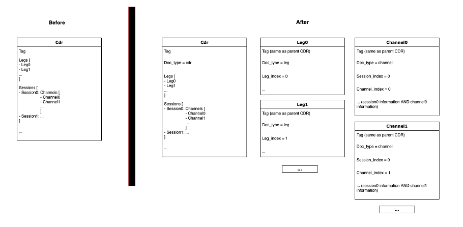
Figure 3: CDR related objects structure
In the screenshot below, (Fig.4), you can see the saved search ExpresswayCdrsSearch opened in the Discover page.
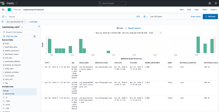
Figure 4: ExpresswayCdrsSearch search in Discover
You can see that this search contains a filter on “doc_type” to only select documents related to CDRs. Kibana will therefore automatically select the fields available for that type of document.
You can expand a document by clicking on the ‘>’ at the beginning of a line, and click on “JSON” to see the full object, as showed in the following screenshot, (Fig. 5):
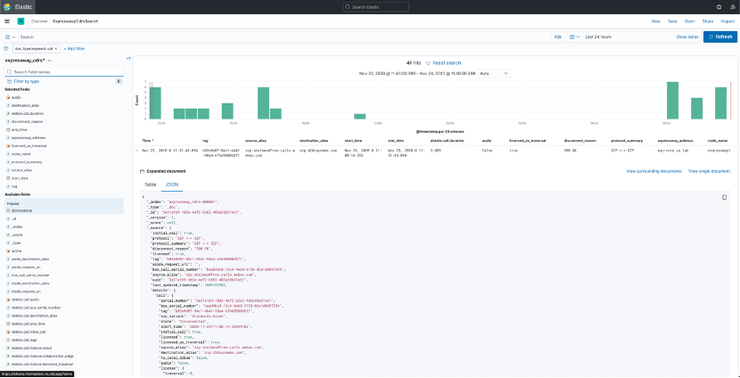
Figure 5: Figure 5: Expanding documents to see JSON object
Here is a description of each type of document in this index pattern:
- CDR: The full object received from Expressway. At the higher level, contains general information about the call, such as the start/end time, the duration, the source/destination alias, the type of license consumed and its unique identifiers (e.g., tag). The CDR object also contains a list of Leg objects, as well as a list of Session objects, which each contain a list of Channel objects.
- Leg: Call legs represent specific sections of a call, and have a direction (ingoing or outgoing). Each object contains information about one call leg, as well as the parent CDR. It contains a “leg_index” value, that indicates its index in the Leg list it is from. It is also contains the same “Tag” value than the CDR it is extracted from, which can be used to link them together.
- Channel: Expressway creates a channel for each component of the call (e.g.,Video, Audio, Content and Signalling), and in both directions (ingoing and outgoing). Each of those channel objects contains information about the media stats, such as the transfer rate, the number of packets transmitted and the number of packets lost. It also contains a “channel_index” value that indicates its index in the list, as well as a “session_index” value.
In an attempt to simplify the already complicated structure, we haven’t created separated Session objects. Instead, each Channel object contains all the information from the parent Session.
Therefore, you can access the session information by accessing any of the Channel object in the list (any channel_index from 0 to 8) and access the “session_*” fields. Those contain information on the requested and allocated bandwidth, as well as the route taken by the call in the different Zones.
Expressway_logs*
(Saved search: ExpresswayLogs)
This index pattern regroups the logs coming from the Expressway nodes via Syslogs messages.
In the screenshot below, (Fig. 6), you can see the saved search ExpresswayLogs opened in the Discover page.
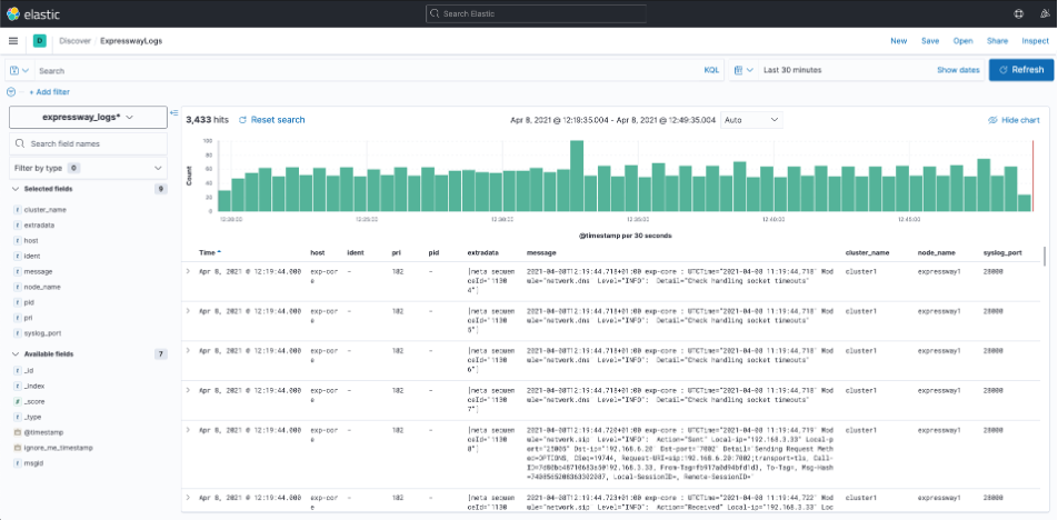
Figure 6: ExpresswayLogs search in Discover
Each log record will contain added information on the source Expressway node. The rest of the fields come from the standard syslog RFC 5424 format. It will contain a “pri” code for each type of log, as well as “ident” that can also help identify what sort of log it is. The full log message is available in the “message” field.
You can search through the logs for a specific term, using the search bar to the left of the time window. The default language supported is KQL (Kibana Query Language), but alternatively you can choose to use Lucene. Make sure to read the documentation on how to search correctly in Kibana in the VQ User Guide and VQ Release Notes. (Chapter title - Kibana Search.)
Cms_logs
(Saved search: CmsLogs)
This index pattern regroups the logs coming from the CMSnodes via Syslogs messages.
In the screenshot below, (Fig. 7), you can see the saved search CmsLogs opened in the Discover page.
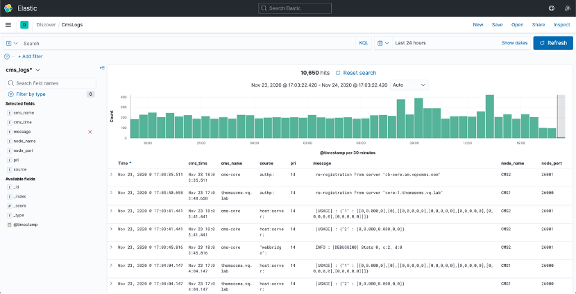
Figure 7: CmsLogs search in Discover
Similarly to the Expressway logs, each record will contain added information on the source CMS node. The CMS syslog messages seem to have they own format, which you can find more details about in the Cisco documentation. It will also contain a “pri” code to identify what type of log it is, as well as the “source” field that indicates the CMS component the log originated from. The log message is available in the “message” field.
Create your own visualisations/dashboards
Now that you have a better understanding of the data coming from your external monitoring sources, you can edit existing visualisations to improve them or adapt them to your use case, or even create your own.
In Kibana 7.10, which is now supported in CM 3.6, a new type of visualisations, Lens, was introduced to make it easier to create visualisations, without needing any Kibana experience or too extensive knowledge of your data.
We have made a video to document this new type of visualisations, and to help you start creating your own visualisations. This video can be viewed from the Analytics area of the Knowldege Base on our Customer Portal. (Search for Analytics or Kibana.)